Keyword Hero enables you to unlock organic search queries on Google. This data provides marketers, SEOs, and web experts with a high level of data-driven insight to make better decisions.
This post will focus on how to analyze keyword overlap between top performing organic and paid keywords. In doing so, this will help you identify where you can optimize your paid keyword efforts.
What is Keyword Overlap?
When you have a dataset of hundreds or even thousands or even thousands of keywords, how can you ensure you are including the best performing organic keywords in your paid campaign?
Well without a solution like Keyword Hero this is simply not possible, as most organic keywords are set to (not provided). Unlocking these organic keywords allows you to identify new opportunities for your paid campaigns.
By selecting the best organic performing keywords for your paid campaign, you may be able to reduce CPC and increase CTR. In addition, as Google awards the top 4 above-the-fold positions to paid AdWords, if you ensure you are ranking there for both paid and organic, then you can increase conversion by taking up more page space.
Organic keywords: when someone searches for something on Google, then that search term is an organic keyword. The higher up your site appears in the rankings, the better this organic keyword is performing for you.
What is the VLOOKUP Function?
V stands for vertical. Basically, the function in Excel or Google Sheets searches columns and returns more information from that row. It is incredibly useful for searching large amounts of keyword data.
We are going to use the VLOOKUP function to create a table containing your top performing organic and paid keywords (AdWords). By analyzing these keywords we will identify new paid keyword opportunities.
Importing the Right Data
First, it is very important to make sure you are importing the correct data.
Please ensure your Keyword Hero property in Google Analytics is configured correctly first. If you are not sure about how to do this, then please check out these resources.
Note that for the first examples, we are going to keep it fairly simple. Each user has a specific use case and more advanced keyword segmentation, but the steps in this guide still apply.
Go to your Keyword Hero Google Analytics property (not your original Google Analytics property).
Organic Keywords: Acquisition > Overview > Organic Search
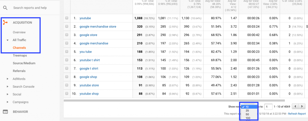
Set your desired time frame and how many rows you want the table of results to show. In this example, we will just choose the first 100 rows of keyword data.
Set the secondary dimension to Position – this is a custom dimension available to Keyword Hero users that allows you to see the Google ranking of a keyword. Learn all about secondary dimensions and custom dimensions.
- Excel users: export this data to a spreadsheet
- Google Sheets users: export this data to a Google Sheet
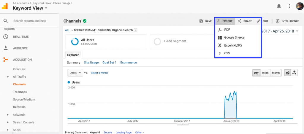
Ok great. Now we have the organic keyword data we need.
Head to your main Google Analytics property (not Keyword Hero). In this step, we are going to export or AdWords data.
Paid Keywords: Acquisition > AdWords > Search Queries
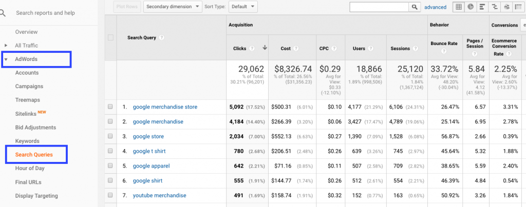
This is very important. If instead, you click on Keywords, you only see the terms you paid for in the campaign–not what people actually clicked on. Clicking on Search Queries shows you the actual results. By default, these paid keywords are listed in order of clicks. Again let’s take the top 100 performing paid keywords.
Make sure you choose a similar timeframe as you did in the organic keywords for more accurate results.
Once again, export this data to Excel or Google Sheets. By default, Google Analytics does not let you export data to the same workbook.
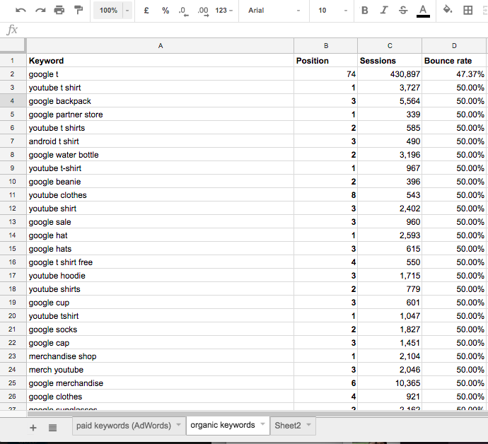
This means you will have to copy and paste the paid data to a new tab in the organic data sheet. The goal is to have both sets of data in the same sheet. In this example, the keyword data has been reduced to just Keyword, Position, Sessions and Bounce Rate. You can include whichever metrics are relevant to your organic keyword data. Finally, we can sort our data by clicking on our desired metric, in this case, bounce rate.
How to Use the VLOOKUP Function
Ok. We are now ready to put the VLOOKUP function to use. Before we do let’s quickly review the syntax of this function (advanced users can skip ahead)
The syntax for the VLOOKUP function is the same in both Google Sheets and Excel:
=VLOOKUP(search term, search range, column to return data from, match type)
- Search term: this is the term we are looking for and can be a number (42), a string “hologram”, or a cell B52.
- Search range: this is the range of cells we are going to search to find our search term. Usually this a column or multiple columns of data.
- Column to return data from: If we search column A for search term “Hologram” we can return the data from Column B associated with this, in this example the definition. This is a number counting from the first column of the range. So column A in a range = 1; B = 2 etc.
- Match type: Setting this to TRUE performs a broad match; setting this to FALSE performs an exact match. For our purposes, we will want to set this to FALSE. By default, this is set to TRUE so don’t forget to change this.
Let’s take a look at a very simple example:
| A | B | C | |
| 1 | Term | Definition | Lookup |
| 2 | Hologram | A three-dimensional image formed by the interference of light beams from a laser or other coherent light source. | =VLOOKUP(“Hologram”, A:B, 2, FALSE) |
Here we query columns A and B for search term “Hologram”. We then return the corresponding information from column 2 (B)
The output in cell C2 is the definition of the term.
- (Full Google Sheets VLOOKUP reference can be found here)
- (Full Excel VLOOKUP reference can be found here)
Using VLOOKUP to Find Keyword Opportunities
Ok, let’s return to the data.
I have named my two tabs of data ‘paid keywords (AdWords)’ and ‘organic keywords’
The column after your data is where we will enter a VLOOKUP formula.
=VLOOKUP(A2, ‘paid keywords (AdWords)’!A:A, 1, FALSE)
This formula takes the cell A2 as our search term. In our case, this is the organic keyword “google t”. It then searches the range in our paid data. To do this we enter the name of that worksheet in single quotes followed by an exclamation mark and the column we want to search. In our case, we want to search column A in the paid keyword data.
Syntax for searching another worksheet tab: ‘Name_of_your_worksheet’!A:A
We set the value to return to ‘1’. We simply want to see if the organic keyword is also present in the paid sheet. If so, then the keyword term will appear in our new column. If it isn’t, ‘#N/A’ will appear instead.
Copy and paste this formula for your data range. Make sure there are no ‘$’ signs. After you hit enter, you can view the results:
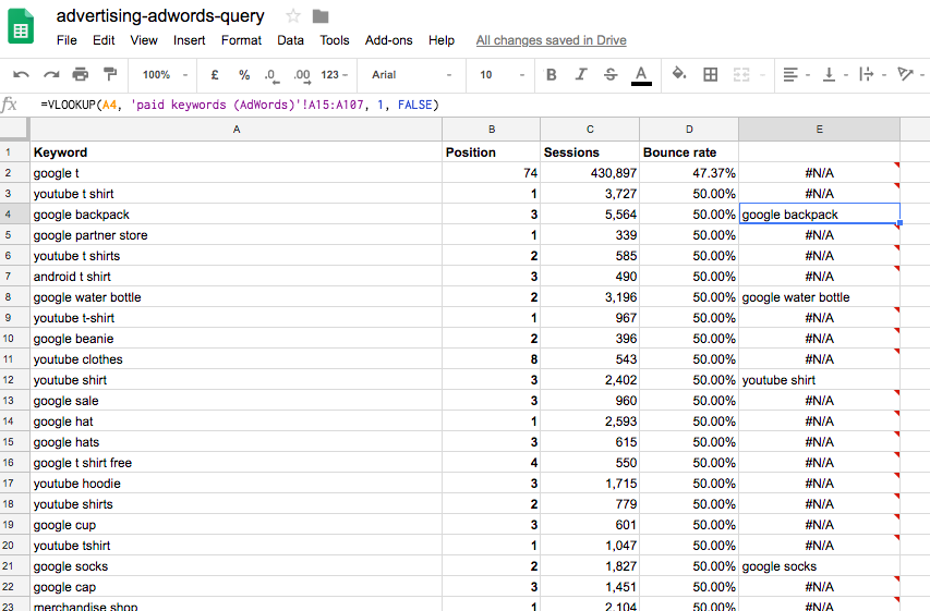
We are looking for organic keywords that are both performing well and that don’t appear in our paid campaign. We have already sorted the data by bounce rate and added custom dimension position.
The organic keyword “youtube t shirt” appears to have a lot of traffic, a low bounce rate and ranks first in the search results. However, this keyword is not included in the paid campaign. Similarly “google hat” has lots of traffic, good bounce rate and is ranking first.
Using this method you can quickly identify paid keyword opportunities.
Try experimenting with VLOOKUP yourself today.
