Logfile analysis allows website owners a deep insight about how Google and other search engines crawl their pages. How often does a bot come by a page, which pages are rarely or not at all visited by the bots? For which pages does the bot get errors? All these and more questions can be answered by a log file analysis.
Unfortunately, a log file analysis is extremely time-consuming in many cases, as very few employees have access to the log files, especially in large organizations. If you have managed to access this treasure trove of data, the evaluation of the usually huge files can cause you headaches.
For collecting our logs we used log-hero.com, a tool which stores the logs directly in Google Analytics and we can simply query the data there via the API and compare this data directly with user data from the main account as needed in the analysis.
Get the Bot Data from Google Analytics
To get to know the paths the google crawler travels along our page, we first need the data provided through Log Hero. We can easily acccess the data through an API call to Google Analyitcs. We like to use the rga package, but you may prefer the googleAnalyticsR. Both deliver the data in the same format, so it’s mostly a matter of personal preference. It is very important though to use the rga package from https://github.com/skardhamar/rga and not it’s capital letter cousin RGA.
rga.open(instance="ga",
client.id = "xxxxxxxxxxxxxx.apps.googleusercontent.com",
client.secret = "xxxxxxxxxxxxxxxxx")
logdata <- ga$getData("177217805", start.date = '2018-06-01', end.date = '2018-10-28', dimensions = "ga:year,ga:date,ga:pagePath", metrics = "ga:hits", filters = "ga:dimension2=@Google;ga:dimension4==200", batch = TRUE
Follow the Googlebot
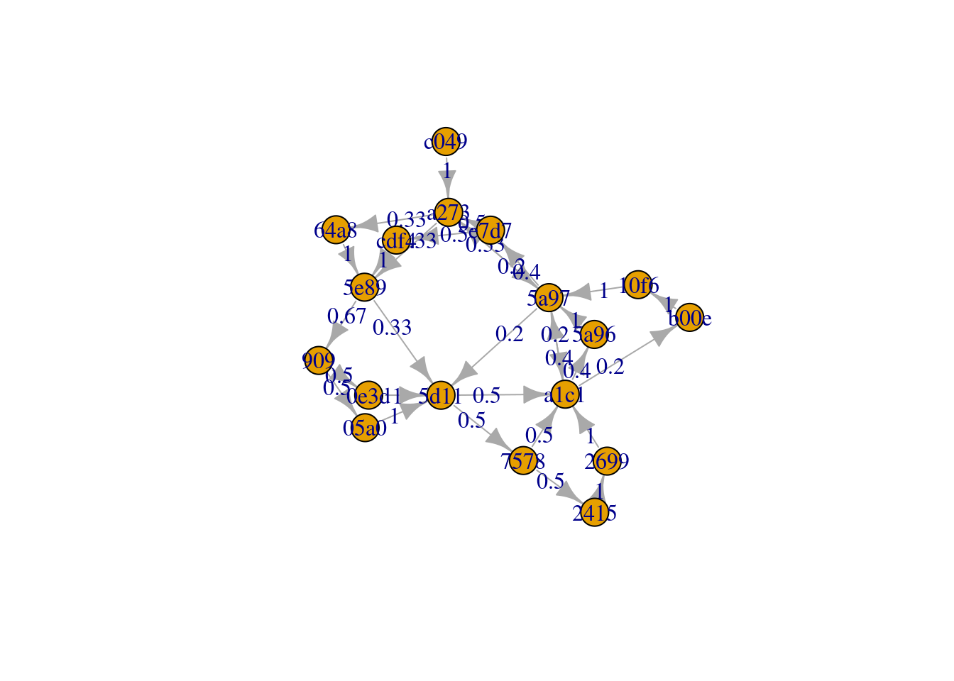
We do some data wrangling to put the steps of the crawler into a format that is accepted by the clickstream package. Now we know the paths the crawlers is taking and are able to find a structure within these paths. A natural model to be applied here is markov chains which are easily fitted and plotted.
# Use four lettters of md4 sum to make plot readable
logdata$pagePathMD5 = substr(unlist(lapply(logdata$pagePath,FUN = digest::sha1)),1,4)
logdata %>%
filter(hits > 10) ->
filtered_logdata# Data wrangling for clickstream format
path <- ddply(filtered_logdata, "year",function(logdata)paste(logdata$pagePathMD5,collapse = ","))
newchar <- as.character(path$V1)
csf <- file(description = "clickstream.txt")
writeLines(newchar,csf)
cls <- readClickstreams(csf, header = TRUE)# Fit and plot MC
mc <- fitMarkovChain(cls)
plot(mc, edge.label = NULL)
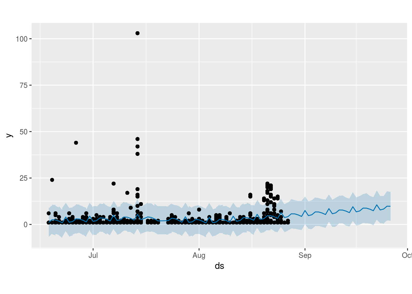
But how often will Google visit us again?
With the help of the high-level prediction package of prophet, we can make easy and surprisingly accurate predictions of how many times the crawler will visit the page in the future – by learning from past data. There is however some erratic component to the crawler behaviour – or rather we are missing some information.
prophet_input = logdata[,c("date","hits")]

colnames(prophet_input)<-c("ds", "y")

m <- prophet(prophet_input)

## Initial log joint probability = -3.33717
## Optimization terminated normally:
## Convergence detected: relative gradient magnitude is below tolerance
future <- make_future_dataframe(m, periods = 60)
forecast <- predict(m, future)
plot(m, forecast)
Estimating the hits of a single page
Now if we add a new page or otherwise want to predcit how often a single page will be visited by the crawler, we would like to build a prediction model. For this, we will use 4 sources of data:
- The Loghero data – Where was the crawler in the past and how often?
- The standard Google Analytics Data – Where and how long do human users stay?
- Screaming Frog page data – Meta data of each page (text ratio, word count, size…)
- Screaming Frog link data – (Unique) in and outlinks to the page
So let us gather all this data. We will be using the googleAnalyticsR package this time.
# GA data
googleAnalyticsR::ga_auth(new_user = TRUE)# Loghero Data
df_loghero = google_analytics_3(id = ">your_LOGHERO_ID<",start = '2018-05-01',end = '2018-10-15',
dimensions = c("ga:dimension2","ga:dimension1", "ga:dimension4" ,"ga:pagePath"),
metrics = c("ga:hits","ga:metric1"),
filters = "ga:dimension2=~^Googlebot(\\-Mobile)?",
samplingLevel = "WALK")# Google Analytics data
df_user_ga = google_analytics_3(id = ">your_GA_ID",start = '2018-05-01',end = '2018-08-15',
dimensions = c("ga:pagePath","ga:hostname"),
metrics = c("ga:pageviews","ga:avgTimeOnPage","entrances"),
samplingLevel = "WALK")# Screaming Frog data
# Written to csv files in screaming frog application
page_data = fread(input = "internal_html.csv")
page_inlinks = fread(input = "all_inlinks.csv")
To merge all our data together we have to do some basic data wrangling.
library(googleAnalyticsR)
library(igraph)
library(ranger)
library(data.table)
library(dplyr)# Feature Engineering and Type Casting
df_loghero$avgMetric1 = df_loghero$metric1 / as.numeric(df_loghero$hits)
df_loghero$hits = as.factor(df_loghero$hits)# Build into a single file
page_data$pagePath = gsub(pattern = "http://ohren-reinigen.de","",page_data$Address)df_loghero$pagePath<-gsub("sitemap", "sitemap",df_loghero$pagePath)
df_loghero$pagePath<-gsub(".*sitemap.*", "sitemap",df_loghero$pagePath)
df_loghero$pagePath<-gsub("^\\/$", "Home",df_loghero$pagePath)df_user_ga$pagePath<-gsub("sitemap", "sitemap",df_user_ga$pagePath)
df_user_ga$pagePath<-gsub(".*sitemap.*", "sitemap",df_user_ga$pagePath)
df_user_ga$pagePath<-gsub("^\\/$", "Home",df_user_ga$pagePath)
# summarise
df_user_ga %>%
group_by(pagePath) %>%
summarise(pageviews = sum(pageviews),
avgTimeOnPage = mean(avgTimeOnPage),
entrances = sum(entrances)) %>%
ungroup() ->
df_user_ga

df_loghero %>%
group_by(pagePath) %>%
summarise(hits = sum(as.numeric(hits)),
avgMetric1 = mean(avgMetric1)) ->
df_loghero
# merge 1
df_merged = merge(page_data, df_loghero, by = "pagePath")
df_merged = merge(df_merged, df_user_ga, by = "pagePath", all.x = TRUE)
# Basic imputation
df_merged$pageviews[is.na(df_merged$pageviews)] = mean(df_merged$pageviews,na.rm = TRUE)
df_merged$avgTimeOnPage[is.na(df_merged$avgTimeOnPage)] = mean(df_merged$avgTimeOnPage,na.rm = TRUE)
df_merged$entrances[is.na(df_merged$entrances)] = mean(df_merged$entrances,na.rm = TRUE)
# Use only R standard variable names
names(df_merged) = make.names(names(df_merged))
We will now use to basic models which we will train on a subset and test on test set. First, we will use a Random Forest to estimate a basic regression, ignoring the ordinal factor scale of counting the visits discreetly, but enjoying the non-linearity. In the second model, we will use a generalize linear model with poisson link and thusly incorporate the fact we are predicting a count variable but losing non-linearity in the proess.
# Modelling
# Train Test Split
train_idx = sample(1:nrow(df_merged),size = round(2*nrow(df_merged)/3),replace = FALSE)
train = df_merged[train_idx,]
test = df_merged[-train_idx,]
# Ranger basic Model
mod_rf = ranger(formula = hits ~ Word.Count
+ Unique.Inlinks
+ Unique.Outlinks
+ Inlinks
+ Outlinks
+ Text.Ratio
+ Response.Time
+ Size
+ pageviews
+ avgTimeOnPage
+ entrances
, data = train, num.trees = 500,importance = "impurity")

mod_glm = glm(formula = hits ~ Word.Count
+ Unique.Inlinks
+ Unique.Outlinks
+ Inlinks
+ Outlinks
+ Text.Ratio
+ Response.Time
+ Size
+ pageviews
+ avgTimeOnPage
+ entrances,
data = train,
family = poisson)
# Predict values
test$pred_rf = round(predict(mod_rf, data = test)$predictions)
test$pred_glm = round(predict(mod_glm, newdata = test))
We have trained the models and now predicted the number of crawler visits for pages the model hast never seen. Let’s compare the predicted values with the actual ones:
test %>%
dplyr::select(pagePath,hits,pred_rf,pred_glm) %>%
arrange(desc(hits))
| pagePath | hits | pred_rf | pred_glm |
|---|---|---|---|
| /ohrenschmalz/ | 197 | 126 | 5 |
| /ohren-reinigen/ohrenkerzen/ | 195 | 74 | 5 |
| /ohren-reinigen/ohren-reinigen-bei-haustieren/ | 127 | 120 | 6 |
| /ohren-reinigen/ohrenreiniger/ | 79 | 72 | 4 |
| /otoskop/ | 69 | 41 | 4 |
| /reinigungsanleitung/ | 63 | 44 | 5 |
| /ohren-reinigen/wattestaebchen/ | 47 | 97 | 4 |
| /testsieger/ | 38 | 53 | 2 |
test %>%
dplyr::select(pagePath,hits,pred_rf,pred_glm) %>%
arrange(desc(hits)) %>%
mutate(rank = rank(1/hits, ties.method = "min"),
rank_rf = rank(1/pred_rf, ties.method = "min"),
rank_glm = rank(1/pred_glm, ties.method = "min")) %>%
dplyr::select(pagePath, rank, rank_rf, rank_glm)
| pagePath | rank | rank_rf | rank_glm |
|---|---|---|---|
| /ohrenschmalz/ | 1 | 1 | 2 |
| /ohren-reinigen/ohrenkerzen/ | 2 | 4 | 2 |
| /ohren-reinigen/ohren-reinigen-bei-haustieren/ | 3 | 2 | 1 |
| /ohren-reinigen/ohrenreiniger/ | 4 | 5 | 5 |
| /otoskop/ | 5 | 8 | 5 |
| /reinigungsanleitung/ | 6 | 7 | 2 |
| /ohren-reinigen/wattestaebchen/ | 7 | 3 | 5 |
| /testsieger/ | 8 | 6 | 8 |
As we can see, the random forest is far more capable of dealing with the large differences in scale in between the pages than the glm. But if we only consider the rank of the pages, both models acutally work pretty well. From an user perspective, the concret number of predicted visits is not as important as the fact which pages are visited more often. The GLM of course offers to take a look at the beta values:
## (Intercept) 11.7771264452 1.884972e+00 6.2479049 4.159949e-10
## Word.Count 0.0063256324 7.856065e-04 8.0519097 8.151201e-16
## Unique.Inlinks 0.0967094083 3.276334e-02 2.9517569 3.159715e-03
## Unique.Outlinks 0.2747712141 1.120261e-01 2.4527436 1.417714e-02
## Inlinks 0.0062746899 6.595578e-03 0.9513481 3.414277e-01
## Outlinks -0.0886505758 4.462267e-02 -1.9866712 4.695885e-02
## Text.Ratio -0.4113764679 7.342136e-02 -5.6029539 2.107293e-08
## Response.Time 2.2484413075 1.285903e+00 1.7485306 8.037219e-02
## Size -0.0002508579 6.675199e-05 -3.7580583 1.712370e-04
## pageviews -0.0004068211 1.399437e-04 -2.9070336 3.648740e-03
## avgTimeOnPage 0.0059767188 1.986728e-03 3.0083225 2.626942e-03
## entrances 0.0004635700 1.624705e-04 2.8532566 4.327367e-03
With these information you can further tune and adjust your homepage and find out what the crawler is actually doing.
Further thoughts to predict the Google Bot
This article shows the first experiments we can do with the data from Log Hero for individual pages. Even further, we managed to produce viable proof-of-concept models for crawler behaviour prediction within a few dozen lines of code. Investing more time and thought may lead to very sophisticate models directly suited to your needs.
The idea now is to add more and more data points to the prediction and to find out what were the most important factors in our prediction – the page speed, behaviour/traffic by real users, in- and outlinks?
We are very happy if you could share your results with us, if you can do similar analyses (or even the same with the code above) analyses or give further tips for perhaps relevant data points.